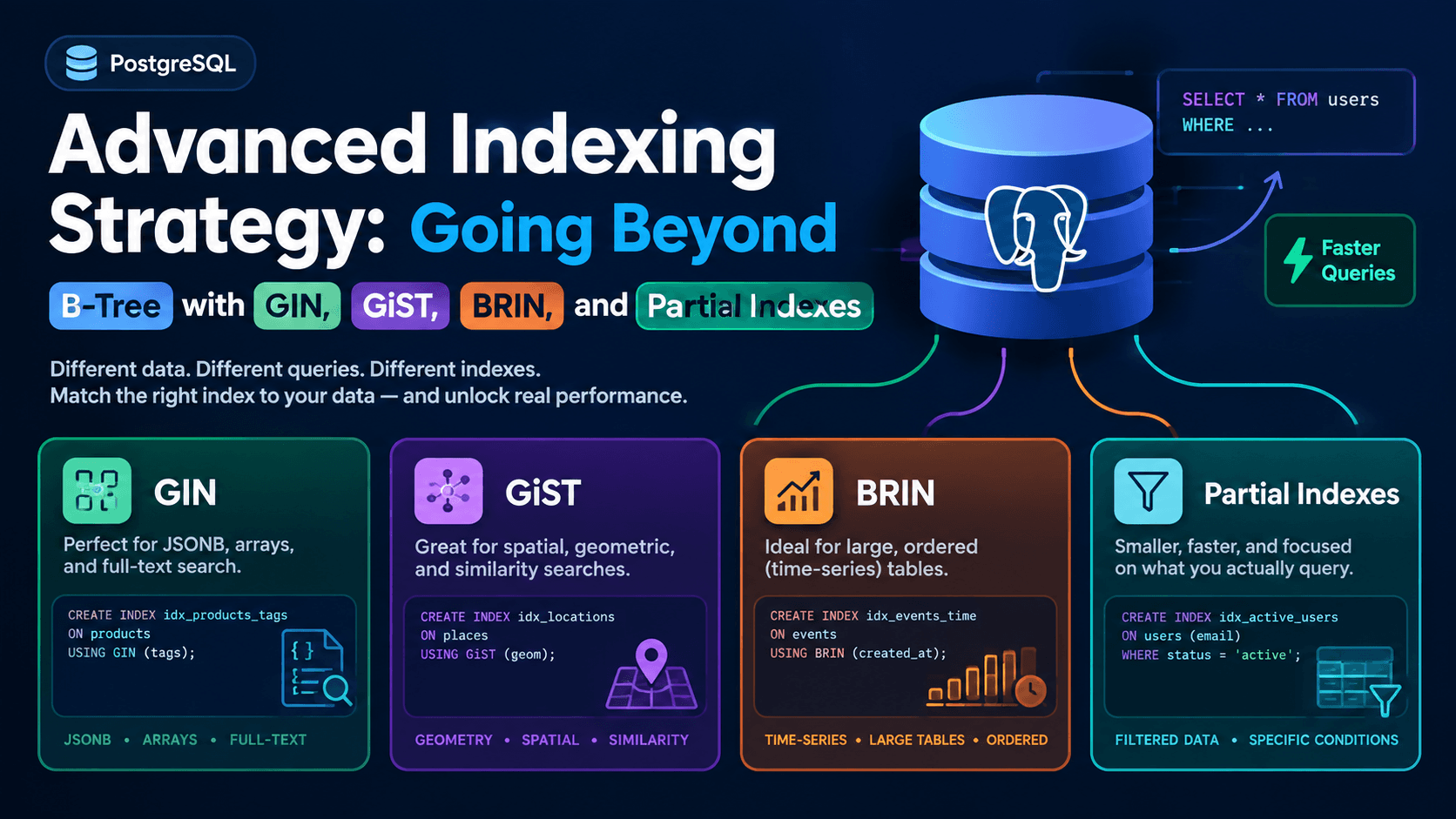
Advanced Indexing Strategy: Going Beyond B-Tree with GIN, GiST, BRIN, and Partial Indexes
If you've worked with a relational database for any length of time, you already know the basic rule: add an index, queries get faster. What most developers don't learn until they hit a real performance wall is that not all indexes are the same tool. The default B-tree index that CREATE INDEX gives you is excellent for equality and range lookups on scalar, well-ordered data — but it's the wrong tool for JSONB documents, full-text search, geometric data, time-series tables, or queries that only ever touch a narrow slice of a huge table.
PostgreSQL ships with several index types specifically because different data shapes and query patterns need fundamentally different underlying data structures. This article walks through when and why to reach for GIN, GiST, BRIN, and partial indexes, with practical examples for each, so you can match the index type to the actual shape of your data instead of defaulting to B-tree everywhere and wondering why the query planner isn't using it.
A Quick Refresher: Why B-Tree Is the Default (and Its Limits)
According to the official PostgreSQL documentation on index types, CREATE INDEX creates a B-tree index by default because it fits the most common situations: equality and range comparisons (, , , , ), , , and / checks on data that can be sorted into a single linear order.
That last phrase — "sorted into a single linear order" — is the key limitation. A B-tree assumes there's one meaningful way to order your values. That assumption breaks down for:
Composite or "contains" data, like JSONB documents, arrays, or full-text documents, where a single scalar ordering doesn't capture the structure.
Multidimensional or overlapping data, like geometric shapes, date ranges, or IP ranges, where "less than" and "greater than" aren't well-defined.
Enormous, naturally-ordered tables, like time-series logs, where a full B-tree is overkill for the actual access pattern.
Queries that only ever touch a small, predictable subset of rows, where indexing the entire table wastes space and write throughput for no query-time benefit.
Each of the four techniques below addresses one of these situations directly.
GIN (Generalized Inverted Index) is built for columns where each row's value effectively contains multiple component values, and your queries ask "does this value contain X?" rather than "is this value greater than X?". Per the official GIN Indexes documentation, GIN maintains a structure similar to an inverted index — for every distinct component value across all rows, it stores which rows contain it — which makes it the natural fit for arrays, JSONB, and text-search vectors.
Example — indexing JSONB for containment queries:
CREATE TABLE products (
  id SERIAL PRIMARY KEY,
  attributes JSONB
);

CREATE INDEX idx_products_attributes_gin
  ON products USING GIN (attributes);

-- This query can now use the GIN index efficiently:
SELECT * FROM products
WHERE attributes @> '{"color": "red", "in_stock": true}';
Example — full-text search:
CREATE TABLE articles (
  id SERIAL PRIMARY KEY,
  body TEXT,
  search_vector tsvector GENERATED ALWAYS AS (to_tsvector('english', body)) STORED
);

CREATE INDEX idx_articles_search_gin
  ON articles USING GIN (search_vector);

SELECT * FROM articles
WHERE search_vector @@ to_tsquery('english', 'database & indexing');
Trade-off to know: GIN indexes are typically larger and slower to update than B-tree indexes, because a single row insertion may need to update many entries in the inverted structure (one per array element, JSON key, or lexeme). PostgreSQL mitigates this with a GIN "pending list" that batches updates, but on write-heavy tables with large JSONB payloads, this overhead is worth measuring before committing to GIN everywhere.
GiST: Indexing Overlaps, Ranges, and Nearest-Neighbor Queries
GiST (Generalized Search Tree) is the tool for data where relationships are about overlap, containment, or distance, rather than strict ordering. The official GiST Indexes documentation describes it as a balanced tree structure that supports arbitrary indexing strategies through user-definable operator classes — which is why it powers geometric types, range types, and nearest-neighbor ("KNN") searches out of the box.
Example — range types (a very common real-world case: booking systems, scheduling, validity periods):
CREATE TABLE room_bookings (
  id SERIAL PRIMARY KEY,
  room_id INT NOT NULL,
  during TSRANGE NOT NULL
);

CREATE INDEX idx_bookings_during_gist
  ON room_bookings USING GIST (during);

-- Find overlapping bookings efficiently — impossible to do this well with a B-tree:
SELECT * FROM room_bookings
WHERE during && '[2026-09-15 09:00, 2026-09-15 11:00)'::tsrange;
You can even enforce "no double-booking a room" directly at the database level using a GiST-backed exclusion constraint:
ALTER TABLE room_bookings
  ADD CONSTRAINT no_overlapping_bookings
  EXCLUDE USING GIST (room_id WITH =, during WITH &&);
Example — nearest-neighbor search on geometric data:
CREATE INDEX idx_locations_geom_gist
  ON store_locations USING GIST (geom);

SELECT name FROM store_locations
ORDER BY geom <-> ST_MakePoint(-0.1276, 51.5074)
LIMIT 5;
GiST and GIN can sometimes both index the same data type (JSONB and arrays, for instance, have GiST operator classes too), but as a rule of thumb: reach for GIN when you need fast lookups and can tolerate slower writes, and reach for GiST when your query needs overlap, containment, or distance semantics, or when you need an exclusion constraint.
BRIN (Block Range Index) solves a completely different problem: not "which structure fits this data type," but "how do I index a table with a billion rows without paying the storage and maintenance cost of a full B-tree?"
The official BRIN Indexes documentation explains that BRIN indexes work by storing summary information — typically the minimum and maximum value — for each range of physically consecutive table blocks, rather than an entry per row. This makes BRIN indexes dramatically smaller than B-tree indexes on the same column, often by one or two orders of magnitude, at the cost of only being effective when a column's values are well-correlated with the physical storage order of the table.
This correlation happens naturally in one very common scenario: append-only, time-ordered data, such as logs, sensor readings, or event tables, where rows are inserted in timestamp order and rarely updated afterward.
Example:
CREATE TABLE sensor_readings (
  id BIGSERIAL PRIMARY KEY,
  recorded_at TIMESTAMPTZ NOT NULL,
  sensor_id INT NOT NULL,
  value NUMERIC
);

-- Table already grows in recorded_at order because rows are appended over time
CREATE INDEX idx_readings_time_brin
  ON sensor_readings USING BRIN (recorded_at);

SELECT AVG(value) FROM sensor_readings
WHERE recorded_at BETWEEN '2026-09-01' AND '2026-09-02';
On a table with hundreds of millions of rows, this BRIN index might be a few hundred kilobytes, compared to gigabytes for an equivalent B-tree — while still letting the planner skip block ranges that fall entirely outside the queried timestamp window. The trade-off is precision: BRIN can only exclude whole block ranges, so queries on columns with poor physical correlation (data that's been reordered by updates, or naturally unordered values like UUIDs) will see little to no benefit and should stick with a B-tree or GIN/GiST index instead.
Partial Indexes: Indexing Only the Rows You Actually Query
The fourth technique isn't a different index type — it's a different index scope. A partial index is built over only the subset of rows that satisfy a WHERE condition, rather than the entire table. The official documentation on partial indexes frames the motivating case clearly: if most queries against a table only ever care about a specific, often small, subset of rows, there's no reason to pay indexing overhead for the rows that are never part of that access pattern.
Classic example — soft-deleted rows:
CREATE TABLE users (
  id SERIAL PRIMARY KEY,
  email TEXT NOT NULL,
  deleted_at TIMESTAMPTZ
);

-- Almost every query in the app filters for active users only:
CREATE UNIQUE INDEX idx_users_email_active
  ON users (email)
  WHERE deleted_at IS NULL;
This index is both smaller (it excludes every deleted row) and enforces uniqueness only among active users — so a deleted user's email address can be reused by a new signup without violating a constraint, which a plain unique index across the whole table cannot express.
Example — indexing only "pending" work items in a large task queue:
CREATE INDEX idx_tasks_pending_priority
  ON tasks (priority DESC, created_at)
  WHERE status = 'pending';
If completed and failed tasks vastly outnumber pending ones, this index stays small and fast even as the tasks table grows into the millions of rows, because it never has to represent rows the application's queue-processing queries don't care about.
Partial indexes combine well with every index type above — you can create a partial GIN index, a partial BRIN index, and so on — and they reduce both storage and the write-time cost of index maintenance, since rows that don't match the WHERE predicate are never added to the index in the first place.
Verifying the Planner Actually Uses Your Index
Creating an index doesn't guarantee PostgreSQL will use it — the query planner makes a cost-based decision, and on small tables a sequential scan is often genuinely faster than an index lookup. The official EXPLAIN documentation describes how to inspect the planner's actual chosen execution plan:
EXPLAIN ANALYZE
SELECT * FROM products
WHERE attributes @> '{"color": "red"}';
Look for Bitmap Index Scan or Index Scan referencing your new index name in the output, rather than Seq Scan. If the planner is still choosing a sequential scan on a table where you'd expect the index to win, common causes include stale table statistics (fixed with ANALYZE tablename;), a query predicate that doesn't match the index's operator class, or a table that's simply still small enough that PostgreSQL's cost estimator prefers scanning it directly.
It's also worth checking whether an index-only scan is possible — a plan that satisfies the entire query from the index structure without touching the table's heap at all — which the documentation on index-only scans notes depends on the queried columns being fully covered by the index and the table's visibility map being up to date (helped by regular VACUUM).
Ranges, geometric data, overlap or nearest-neighbor queries
GiST
Huge, append-only, naturally time-ordered tables
BRIN
Queries that only ever touch a known, narrow subset of rows
Partial index (any type)
In practice, production schemas usually combine these rather than picking just one — a deleted_at IS NULL partial index alongside a GIN index on a JSONB column, or a BRIN index on created_at alongside a B-tree on a foreign key, are both completely normal and often necessary for a table serving several distinct query patterns well.
Key Takeaways
The default B-tree index is a good starting point, but treating it as the only option leaves significant performance on the table for JSONB, full-text, geometric, and time-series workloads. GIN excels at "does this contain X" queries on composite data. GiST handles overlap, range, and distance-based queries that a linear ordering can't express. BRIN trades precision for a dramatic reduction in index size on enormous, naturally-ordered tables. And partial indexes let you index exactly the rows your application actually queries, regardless of which underlying index type you choose. Matching the index type to the actual shape of your data — and confirming the choice with EXPLAIN ANALYZE rather than assuming — is what separates a database that scales gracefully from one that quietly falls back to sequential scans as it grows.
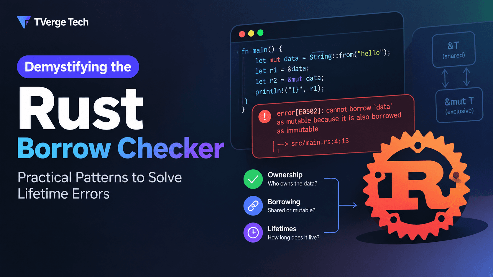
3Demystifying the Rust Borrow Checker: Fix Lifetime Errors Fast